Isotopic calculations
APAV supports the computation of elemental and molecular isotope distributions. These calculations are important to most mass spectrum analysis and indexing operations. Elemental isotopes are typically quite easy to access as they are tabulated in most periodic table resources (i.e. websites, Cameca poster), however molecular isotopes are not so easily determined. Molecular isotopes are computed based on the elemental composition and isotopic distribution of the molecules constituents.
The calculation is combinatorial in nature and can drastically increase in computation time the more complex the molecule is (combinatorial explosion). However, the molecules likely to be found in an atom probe experiment are not so complex for this is to be problematic, the computations will be more or less instant.
The principle class is IsotopeSeries, signifying that it produces a series of isotopes corresponding to the given composition. As a simple example, get the isotopes of singly charged elemental copper:
>>> import apav as ap
>>> cu_isos = ap.IsotopeSeries("Cu", 1)
>>> print(cu_isos)
IsotopeSeries: Cu +1, threshold: 1.0%
    Ion      Isotope     Mass    Abs. abundance %    Rel. abundance %
--  -----  ---------  -------  ------------------  ------------------
 1  Cu            63  62.9296               69.17            100
 2  Cu            65  64.9278               30.83             44.5713
Under the hood, APAV uses Ion objects to represent the ions or compositions. This code snippet does the same thing:
>>> cu_isos = ap.IsotopeSeries(ap.Ion("Cu", 1)):
>>> print(cu_isos)
IsotopeSeries: Cu +1, threshold: 1.0%
    Ion      Isotope     Mass    Abs. abundance %    Rel. abundance %
--  -----  ---------  -------  ------------------  ------------------
 1  Cu            63  62.9296               69.17            100
 2  Cu            65  64.9278               30.83             44.5713
The list of the isotopes (each isotope is an Isotope) can be access with:
>>> cu_isos.isotopes
[Isotope: Cu +1 63 @ 62.93 Da 69.17 %, Isotope: Cu +1 65 @ 64.928 Da 30.83 %]
The calculation for molecular isotopes is the same, i.e. for CuO2:
>>> import apav as ap
>>> ap.IsotopeSeries("CuO2", 1)
IsotopeSeries: CuO2 +1, threshold: 1.0%
    Ion      Isotope     Mass    Abs. abundance %    Rel. abundance %
--  -----  ---------  -------  ------------------  ------------------
 1  CuO2          95  94.9194             68.8342            100
 2  CuO2          97  96.9176             30.6803             44.5713
In this way isotopic information of arbitrary compositions can be queried. Atom probe uses time of flight mass spectrometry which means that the mass spectrum is also sensitive to the charge. This means that the spectrum of a cuprate oxide material may exhibit both CuO2 1+ as well as CuO2 2+, resulting in two sets of CuO2 peaks that are shifted according to the charge (mass/charge ratio). The charge can be changed to produce the CuO2 2+ set of isotopes:
>>> import apav as ap
>>> ap.IsotopeSeries("CuO2", 2)
IsotopeSeries: CuO2 +2, threshold: 1.0%
    Ion      Isotope     Mass    Abs. abundance %    Rel. abundance %
--  -----  ---------  -------  ------------------  ------------------
 1  CuO2          95  47.4597             68.8342            100
 2  CuO2          97  48.4588             30.6803             44.5713
Here the theoretical mass/charge ratios are half of the singly charged isotopes, given the doubly charged ion. Now one might notice that the total absolute abundance does not add up to 100%. This is because the isotopes displayed are thresholded by the absolute abundance. This is done to prevent large amounts of isotopes with more complex molecular structures. Take a SnO2 2+ for example, Sn has 10 natural isotopes and oxygen has 3, this eventually produces 60 possible isotopes. If we set the threshold value to 0 all of these isotopes will be generated:
>>> import apav as ap
>>> SnO2_isos = ap.IsotopeSeries("SnO2", 2, threshold=0)
>>> len(SnO2_isos)
60
Showing all of the isotopes:
>>> print(sno2_isos)
IsotopeSeries: O2Sn +2, all isotopes
    Ion      Isotope     Mass    Abs. abundance %    Rel. abundance %
--  -----  ---------  -------  ------------------  ------------------
 1  O2Sn         144  71.9473         0.965292            2.97729
 2  O2Sn         145  72.4494         0.000735409         0.00226825
 3  O2Sn         146  72.9463         0.656796            2.02578
 4  O2Sn         146  72.9494         0.00396734          0.0122366
 5  O2Sn         146  72.9515         1.40068e-07         4.32017e-07
 6  O2Sn         147  73.4466         0.33835             1.04359
 7  O2Sn         147  73.4484         0.000500381         0.00154335
 8  O2Sn         147  73.4516         1.51126e-06         4.66124e-06
 9  O2Sn         148  73.9458        14.4694             44.6286
10  O2Sn         148  73.9484         0.00269942          0.00832594
11  O2Sn         148  73.9487         0.000257772         0.000795057
12  O2Sn         148  73.9505         9.5304e-08          2.9395e-07
13  O2Sn         148  73.9516         4.07642e-06         1.25731e-05
14  O2Sn         149  74.4464         7.64272            23.5727
15  O2Sn         149  74.4479         0.0110235           0.0340004
16  O2Sn         149  74.4487         0.00139061          0.00428912
17  O2Sn         149  74.4505         1.02828e-06         3.17156e-06
18  O2Sn         149  74.4508         4.9096e-08          1.51429e-07
19  O2Sn         150  74.9457        24.1024             74.3401
20  O2Sn         150  74.9479         0.0594691           0.183423
21  O2Sn         150  74.9485         0.00582262          0.0179589
22  O2Sn         150  74.95           2.09958e-06         6.4758e-06
23  O2Sn         150  74.9506         2.77365e-06         8.55488e-06
24  O2Sn         150  74.9508         5.2972e-07          1.63384e-06
25  O2Sn         151  75.4466         8.5483             26.3659
26  O2Sn         151  75.4478         0.0183625           0.0566361
27  O2Sn         151  75.4485         0.0314115           0.0968837
28  O2Sn         151  75.45           2.26533e-05         6.98705e-05
29  O2Sn         151  75.4506         1.10899e-06         3.42051e-06
30  O2Sn         151  75.4508         1.42885e-06         4.40706e-06
31  O2Sn         152  75.946         32.4219            100
32  O2Sn         152  75.9478         0.0990607           0.305537
33  O2Sn         152  75.9487         0.00651254          0.0200869
34  O2Sn         152  75.9499         3.49737e-06         1.07871e-05
35  O2Sn         152  75.95           6.11043e-05         0.000188467
36  O2Sn         152  75.9506         1.19654e-05         3.69055e-05
37  O2Sn         153  76.4481         0.0247006           0.0761851
38  O2Sn         153  76.4487         0.0351334           0.108363
39  O2Sn         153  76.4499         3.77348e-05         0.000116387
40  O2Sn         153  76.4506         3.22752e-05         9.95477e-05
41  O2Sn         153  76.4508         1.2404e-06          3.8258e-06
42  O2Sn         154  76.9466         4.60753            14.2112
43  O2Sn         154  76.9481         0.133253            0.410999
44  O2Sn         154  76.95           0.000101785         0.000313938
45  O2Sn         154  76.9502         4.70455e-06         1.45104e-05
46  O2Sn         154  76.9508         1.33832e-05         4.12784e-05
47  O2Sn         155  77.4487         0.00351025          0.0108268
48  O2Sn         155  77.4502         5.07596e-05         0.00015656
49  O2Sn         155  77.4508         3.60995e-05         0.000111343
50  O2Sn         156  77.9476         5.76189            17.7716
51  O2Sn         156  77.9488         0.0189369           0.0584077
52  O2Sn         156  77.9503         0.000136917         0.0004223
53  O2Sn         156  77.9509         6.68572e-07         2.0621e-06
54  O2Sn         157  78.4497         0.00438971          0.0135393
55  O2Sn         157  78.4509         7.21354e-06         2.2249e-05
56  O2Sn         158  78.9497         0.0236813           0.0730412
57  O2Sn         158  78.9509         1.94576e-05         6.00138e-05
58  O2Sn         158  78.9518         8.36076e-07         2.57874e-06
59  O2Sn         159  79.4518         9.02082e-06         2.78233e-05
60  O2Sn         160  79.9518         2.43325e-05         7.50496e-05
We can iterate through all of the isotopes (each isotope is a Isotope instance) and count the number of isotopes that are less than 1% absolute abundance:
>>> count = sum(1 for i in iso if i.abundance < 0.01)
>>> print(count)
53
So 53 out of 60 isotopes are less than 1% theoretical abundance. Looking at the list above, many are considerably below that value. Thus, the default threshold for IsotopeSeries is 1%:
>>> ap.IsotopeSeries("SnO2", 2)
IsotopeSeries: O2Sn +2, threshold: 1.0%
    Ion      Isotope     Mass    Abs. abundance %    Rel. abundance %
--  -----  ---------  -------  ------------------  ------------------
 1  O2Sn         148  73.9458            14.4694              44.6286
 2  O2Sn         149  74.4464             7.64272             23.5727
 3  O2Sn         150  74.9457            24.1024              74.3401
 4  O2Sn         151  75.4466             8.5483              26.3659
 5  O2Sn         152  75.946             32.4219             100
 6  O2Sn         154  76.9466             4.60753             14.2112
 7  O2Sn         156  77.9476             5.76189             17.7716
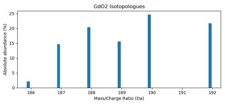
Gives all isotopes >1% abundance. This default value was chosen as it is unlikely to have enough counts in the limited statistical size of atom probe experiments to resolve smaller probabilities. The isotope distribution can be visualized using matplotlib:
>>> import apav as ap
>>> import matplotlib.pyplot as plt
>>> GdO2_isos = ap.IsotopeSeries("GdO2", 1)
>>> plt.bar(GdO2_isos.masses, GdO2_isos.abundances*100, width=0.1)
>>> plt.xlabel("Mass/Charge Ratio (Da)")
>>> plt.ylabel("Absolute abundance (%)")
>>> plt.title("GdO2 Isotopologues")
>>> plt.show()