Spectrum analysis
Computing compositions from mass spectra (or directly from the ion list) are a central component to APT experiments. Every mass spectrum is different, with varying levels of background and therm tails. APAV supports 3 different methods for quantifying mass spectra, with additive amounts of background correction. All mass spectrum analyses are imported from apav.analysis.
Quantifying with no corrections
Without applying any background fitting/corrections, we can compute compositions by just adding up all ions of range. This done using RangedMassSpectrum where by counts between specified ranges in a RangeCollection are counted, assigned to compositions, and then the composition is calculated. No fitting or correction of any kind is applied using RangedMassSpectrum. This quantification method does not actually use binned histograms for the computation, so the counts calculated here are exact (statistically exact, not compositionally).
Using the GdBa2Cu3O7 Roi again, we can compute the composition using RangedMassSpectrum using a greatly simplified set of ranges:
>>> import apav as ap
>>> import apav.analysis as anl

>>> # Load the POS data
>>> roi = ap.Roi.from_pos("GBCO.pos")

>>> # Create a few ranges, the color is used in plotting the spectrum
>>> rngs = [ap.Range("O2", (31.9, 33.5), color=(1, 0, 0)),
>>>        ap.Range("Cu", (62.8, 66.6), color=(0, 1, 0)),
>>>        ap.Range("Gd", (50, 56), color=(0, 0, 1)),
>>>        ap.Range("Ba", (66.9, 70), color=(1, 0, 1))]

>>> rng_col = ap.RangeCollection(rngs)

>>> # Create the ranged mass spectrum
>>> mass_quant = anl.RangedMassSpectrum(roi, rng_col, percent=True)
Now print the results of the quantification with RangedMassSpectrum.print().
>>> ranged_mass.print()
Ion      Composition    Counts
-----  -------------  --------
O2          38.1431   15537944
Cu          27.6362   11257848
Gd           5.14616   2096333
Ba          29.0745   11843781
We can get the quantification data as a dictionary:
>>> comp = mass_quant.quant_dict
>>> comp["Cu"]
(27.636179246878662, 11257848)
It is usually more helpful to compute the composition using the decomposition of polyatomic ions. This is simply a flag in RangedMassSpectrum:
>>> mass_quant = anl.RangedMassSpectrum(roi, rng_col, percent=True, decompose=True)
>>> mass_quant.print()
Ion      Composition       Counts
-----  -------------  -----------
O           55.2226   3.10759e+07
Cu          20.0055   1.12578e+07
Gd           3.72523  2.09633e+06
Ba          21.0467   1.18438e+07
As a result, the “O2” in our results changed to “O” and the counts doubled, since each O2 ion contributes 2 counts to the O concentration. This composition is obviously inaccurate, we have greatly simplified the ranging structure for the sake of example.
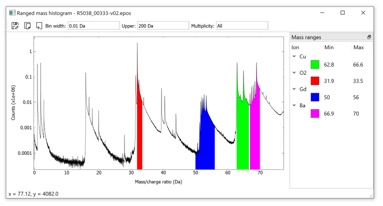
Plotting the uncorrected mass spectrum
We can interactively plot the mass spectrum to assess the validity of our ranging:
>>> plot = ranged_mass.plot()
>>> plot.show()
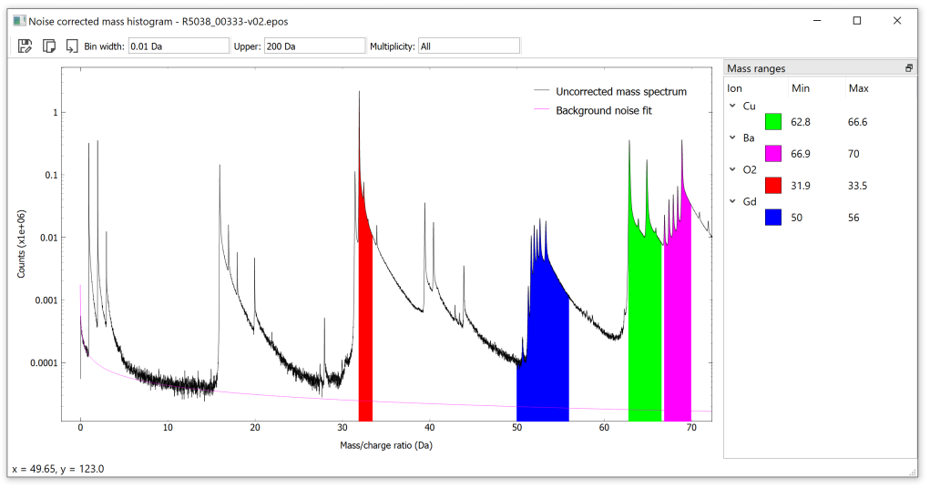
Noise corrected mass spectrum
The NoiseCorrectedMassSpectrum is the first tier of corrections that can be applied to mass spectra. Here the “random noise” background of the mass spectrum is fit and subtracted. This is typically done by fitting a decay function to the initial part of the binned mass histogram before the first hydrogen peak. The “random noise” background arises from field ionization of particles in the vacuum that happen to get sufficiently close to the specimen apex.
Note
If no fit interval is provided, a default is used. This default interval does not always match due to variations in where the first counts start in a spectrum. If encountering errors, this fit interval should be the first thing check.
Again using GBCO.pos:
>>> import apav.analysis as anl
>>> import apav as ap

>>> rngs = [ap.Range("O2", (31.9, 33.5), color=(1, 0, 0)),
>>>        ap.Range("Cu", (62.8, 66.6), color=(0, 1, 0)),
>>>        ap.Range("Gd", (50, 56), color=(0, 0, 1)),
>>>        ap.Range("Ba", (66.9, 70), color=(1, 0, 1))]
>>> rng_col = ap.RangeCollection(rngs)
Printing the results:
>>> mass_quant = anl.NoiseCorrectedMassSpectrum(roi, rng_col, percent=True, decompose=True)
>>> mass_quant.print()
Ion      Composition       Counts
-----  -------------  -----------
O           55.2395   3.1068e+07
Cu          20.0048   1.12512e+07
Gd           3.70669  2.08473e+06
Ba          21.049    1.18385e+07
The change in composition due to the noise correction is very little. This because this specimen was evaporated at a moderate laser energy which naturally reduces the noise background due to the lower fields at the apex. Specimens evaporated at lower laser energies, or specimens that are voltage pulsed, will have much larger noise background where correction because more important. Instead, higher laser energies produce larger thermal tails, which is where local background subtraction (using LocalBkgCorrectedMassSpectrum) increases in importance.
The mass spectrum can be plot to assess the fit to the noise background:
>>> plot = mass_quant.plot()
>>> plot.show()
Backgrounds
The background fitting can be controlled for NoiseCorrectedMassSpectrum and LocalBkgCorrectedMassSpectrum, though the random noise fit should work out of the box without manual intervention (maybe except cases where the systems mass spectrum calibration is bad and requires much correction at reconstruction).
As an example we will do the same noise corrected quantification, but fit the noise background on the last hydrogen isotope tail and the last 5 Daltons of the data set (195-200 Da) to show how backgrounds can be fit on multiple non-contiguous intervals.
Backgrounds are defined using the Background class, and the mathematical models are borrowed from lmfit. To define a background that fits on the interval [3.06, 9] using a exponential decay:
>>> from apav.analysis import models
>>> import apav.analysis as anl
>>> from lmfit.models import ExponentialModel

>>> new_bkg = anl.Background((3.06, 9), model=ExponentialModel())
The Background will take any Model from lmfit, custom models may also be used as long as it implements Model.guess(). APAV defines a few extra models in apav.analysis.models to account for things like shifting, as well as better boundary and initial values. To redo the noise corrected quantification using our new background:
>>> import apav as ap
>>> import apav.analysis as anl
>>> from lmfit.models import ExponentialModel

>>> # Load the POS data
>>> roi = ap.Roi.from_pos("GBCO.pos")

>>> # Create a few ranges, the color is used in plotting the spectrum
>>> rngs = [ap.Range("O2", (31.9, 33.5), color=(1, 0, 0)),
>>>        ap.Range("Cu", (62.8, 66.6), color=(0, 1, 0)),
>>>        ap.Range("Gd", (50, 56), color=(0, 0, 1)),
>>>        ap.Range("Ba", (66.9, 70), color=(1, 0, 1))]

>>> rng_col = ap.RangeCollection(rngs)

>>> # Create the ranged mass spectrum
>>> new_bkg = anl.Background([(3.06, 9)], model=ExponentialModel())
>>> mass_quant = anl.NoiseCorrectedMassSpectrum(roi,
>>>                                     rng_col,
>>>                                     percent=True,
>>>                                     decompose=True,
>>>                                     noise_background=new_bkg)
Plotting our new background:
>>> plot = mass_quant.plot()
>>> plot.show()
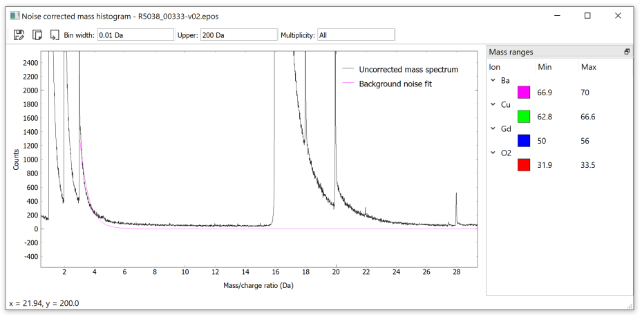
This has successfully done a noise corrected background using an exponential decay on the hydrogen isotope at 3 Da. The fit is not very good, the exponential decay function does not model the tailing edges of mass spectrum peaks as well as the power law; but this shows how to change the Background.
If more detail about the fit is desired, the lmfit ModelResult can be accessed by Background_fit_result. Note that this will be None if the background has not been fit yet (which is typically handled by NoiseCorrectedMassSpectrum or LocalBkgCorrectedMassSpectrum.
Background collections
To handle having multiple background models, intervals, etc for selected ranges, a new container is introduced to handle multiple backgrounds, the BackgroundCollection. For example, if we had two asymmetric peaks with long tailing edges (as is common with laser-assisted evaporation) at 63 and 65 da, we could define separate backgrounds for each peak as:
>>> import apav.analysis as anl
>>> from apav.analysis import models
>>> bkgs = anl.BackgroundCollection()
>>> bkgs.add(anl.Background((60, 62.5),
>>>                         include_intervals=(62, 64),
>>>                         model=models.PowerLawShiftModel()))
>>> bkgs.add(anl.Background((63.5, 64.5),
>>>                         include_intervals=(64, 66),
>>>                         model=models.PowerLawShiftModel()))
We can add any number of backgrounds as needed. One of the key components here is the include_intervals parameter. This defines a single, or multiple half-open intervals that maps each Background to zero or more Range (ranges). This allows a single Background to be applied to any number of ranges. The LocalBkgCorrectedMassSpectrum takes each include interval and searches each Range for matches. A Range matches to a Background’s include interval(s) if the lower bound of the Range is contained within the include_interval. For example, we can define a single Background and apply it to each of these theoretical. First define the ranges, for the 63 Da peak we will define the range [62.5, 63.5) and for 65 Da [64.5, 65.5):
>>> import apav.analysis as anl
>>> from apav.analysis import models
>>> rngs = ap.RangeCollection()
>>> rngs.add(ap.Range("Cu", (62.5, 63.5)))
>>> rngs.add(ap.Range("Cu", (64.5, 65.5)))
Then we define a single background that fits a displaced power law from 60 to 62.5 Da. This has the include interval from 62-66 Da, meaning any Range with Range.lower in the interval [62, 66) will be background subtracted using this single background. In this case, both of these Range use the same background:
>>> bkgs = anl.BackgroundCollection()
>>> bkgs.add(anl.Background((60, 62.5),
>>>                         include_intervals=(62, 66),
>>>                         model=models.PowerLawShiftModel()))
Generally power laws fit mass spectrum tails sufficiently well, although sometimes a tail may fit better with a different shape (due to any number of factors), the background models can be mixed and matched. For example to define the first background as power law and the second as a lorentzian:
>>> bkgs = anl.BackgroundCollection()
>>> bkgs.add(anl.Background((60, 62.5),
>>>                         include_intervals=(62, 64),
>>>                         model=models.PowerLawShiftModel()))
>>> from lmfit.models import LorentzianModel
>>> bkgs.add(anl.Background((63.5, 64.5),
>>>                         include_intervals=(64, 66),
>>>                         model=LorentzianModel()))
In principle any model from lmfit.models could be used, although one must consider how well a shape can fit the data, not all shapes may converge to a solution. Custom models can be made when needed by subclassing lmfit.models.Model, with the only requirements that Model.guess() is defined to provide initial values, and boundaries, as weell as the model itself defined. See apav.analysis.models.PowerLawShiftModel for an example, which was defined for use in APAV.
Local background subtracted mass spectrum
The LocalBkgCorrectedMassSpectrum is the final tier of corrections that can be applied to a mass spectrum. This scheme first applies the random noise background correction, then applies local background fitting and subtraction to specified areas or peaks in the binned mass histogram. There is no constraint imposed that ranges must be background corrected. In fact, if no local background fits are defined the result is the exact same as the NoiseCorrectedMassSpectrum.
Due to the close proximity of peaks and tails in complex systems it may not be realistic to apply separate background fits to close peaks. This class separates background fits from ranges so that a single background fit can be easily applied to multiple ranges, or the model changed for a problematic tail shape. This way the background correction of the mass spectrum can be completely controlled.
Using our previous example with NoiseCorrectedMassSpectrum lets extend this with local background correction. First setup the imports, Roi, and RangeCollection:
import apav.analysis as anl
import apav as ap
roi = Roi.from_pos("GBCO.pos")
rng_lst = [ap.Range("O2", (31.9, 33.5), color=(1, 0, 0)),
           ap.Range("Cu", (62.8, 66.6), color=(0, 1, 0)),
           ap.Range("Gd", (50, 56), color=(0, 0, 1)),
           ap.Range("Ba", (66.9, 70), color=(1, 0, 1))]
rngs = ap.RangeCollection(rng_col)
Now the BackgroundCollection:
bkgs = anl.BackgroundCollection()
bkgs.add(anl.Background((22, 24), include_interval=(30, 35)))  # O2 background
bkgs.add(anl.Background((45, 49), include_interval=(45, 55)))  # Gd background
bkgs.add(anl.Background((55, 60), include_interval=(60, 63)))  # Cu background
bkgs.add(anl.Background((66.1, 66.7), include_interval=(63, 70)))  # Ba background
The include_intervals keyword can be forgone for brevity, but it is included for clarity. Now for the LocalBkgCorrectionMassSpectrum:
>>> mass_quant = anl.LocalBkgCorrectedMassSpectrum(roi, rngs, bkgs, percent=True, decompose=True)
>>> mass_quant.print()
Ion      Composition       Counts
-----  -------------  -----------
O           56.4777   3.10669e+07
Cu          20.3612   1.12002e+07
Gd           3.72177  2.04725e+06
Ba          19.4393   1.06931e+07
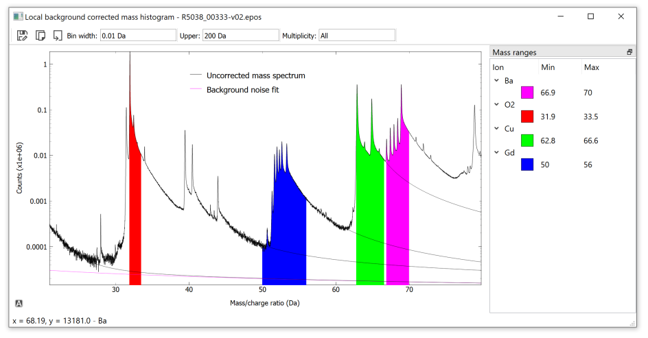
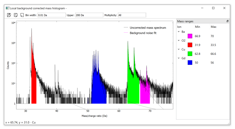
Here we see that the concentration of oxygen has increased by ~ 1.2at% (compared to the noise corrected quantification) with all other elements decreasing. This makes sense as there is more background under the Ba, Cu, and Gd mass ranges than the O2 range. We can assess this visually by using the interactive plotter, while also looking at the quality of the fits:
>>> plot = mass_quant.plot()
>>> plot.show()
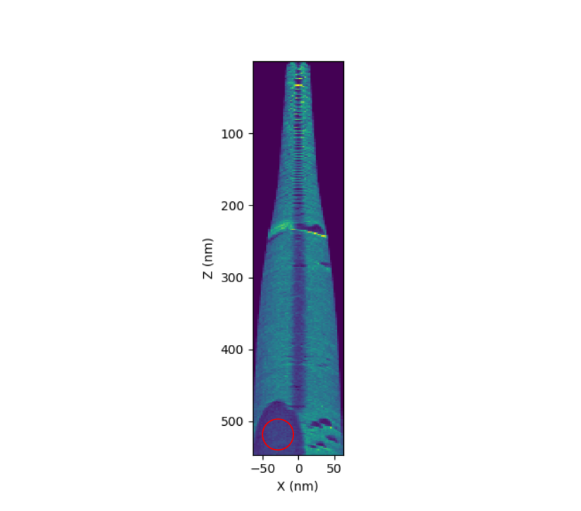
Measuring the composition of a precipitate
The composition of a precipitate (or any other subset of the Roi) can be calculated by combining the mass spectrum analyses capability with Roi subsets, such as RoiSphere. In our GBCO example, we have a small precipitate near the bottom of the reconstruction:
In order to compute the local background-subtracted composition of this precipitate, all we have to do is pass the RoiSphere to LocalBkgCorrectedMassSpectrum instead of the entire Roi. All of this becomes:
>>> # Ranges
>>> rng_lst = [ap.Range("O2", (31.9, 33.5), color=(1, 0, 0)),
>>>        ap.Range("Cu", (62.8, 66.6), color=(0, 1, 0)),
>>>        ap.Range("Gd", (50, 56), color=(0, 0, 1)),
>>>        ap.Range("Ba", (66.9, 70), color=(1, 0, 1))]
>>> rngs = ap.RangeCollection(rng_lst)

>>> # Backgrounds
>>> bkgs = anl.BackgroundCollection()
>>> bkgs.add(anl.Background((22, 24), include_interval=(30, 35)))  # O2 background
>>> bkgs.add(anl.Background((45, 49), include_interval=(45, 55)))  # Gd background
>>> bkgs.add(anl.Background((55, 60), include_interval=(60, 63)))  # Cu background
>>> bkgs.add(anl.Background((66.1, 66.7), include_interval=(63, 70)))  # Ba background

>>> # Extract the counts in a sphere within the precipitate
>>> sphere = ap.RoiSphere(roi, (-30, 0, 520), 20)

>>> # Quantification
>>> mass_quant = anl.LocalBkgCorrectedMassSpectrum(sphere, rngs, bkgs, percent=True, decompose=True)
>>> mass_quant.print()
Ion      Composition    Counts
-----  -------------  --------
O           64.179      125556
Cu          21.1057      41290
Gd          13.2932      26006
Ba           1.42204      2782
So we have found that the precipitate is a Barium deficient composition, though we would need to range more of the to make better quantitative judgements. Now plot the spectrum to determine the fit quality:
The lower number of counts has made the fits slightly worse, but this to be expected. And we can see the elimination of the Ba isotopes, with exception of one peak. If we check the Ba isotopes we can determine if this is an actual residual Barium isotope, or if it is a lower intensity peak belonging to some other composition:
>>> ap.IsotopeSeries("Ba", 2)
IsotopeSeries: Ba +2, threshold: 1.0%
    Ion      Isotope     Mass    Abs. abundance %    Rel. abundance %
--  -----  ---------  -------  ------------------  ------------------
 1  Ba           134  66.9523               2.417             3.37108
 2  Ba           135  67.4528               6.592             9.19412
 3  Ba           136  67.9523               7.854            10.9543
 4  Ba           137  68.4529              11.232            15.6657
 5  Ba           138  68.9526              71.698           100
Comparing these isotopes to the Ba area of the spectrum, we can assert that the residual peak belongs to the most abundant Ba isotope at ~69 Da, so this peak should still be ranged as barium.
Laser energy dependency
It is commonplace in literature to compute the laser energy dependence of mass spectrum quantification. This is usually performed by either evaporating multiple specimens at steadily increasing (or decreasing) laser energies, or evaporating a single specimen and periodically increasing/decreasing the laser energy in-situ (more commonly). Additionally, the charge ratio of a particular ion is sometimes of interest, and how it evolves over laser energies. APAV can be used to more easily automate the process of computing these mass spectra changes with the evolution of laser energy.
As an example, suppose we have field evaporated a single specimen of GdBa2Cu3O7 and varied the laser energy from 50pJ down to 0.05pJ. Each portion of the reconstruction constituting a particular wavelength was reconstructed and saved as a separate POS file. Using these POS file and either an RNG/RRNG file (or constructing one manually) we can compute the composition as a function of laser energy. Using the same sample ranges and backgrounds as we have used in previous sections:
# Imports
import apav as ap
import apav.analysis as anl
from apav.analysis import models
from collections import OrderedDict
import matplotlib.pyplot as plt
import numpy as n

# The (Energy: roi path) key/value pairs, mapping the laser energy to the POS path
roi_paths = OrderedDict([
    (50, r"R5038_00335-v02-roi-50.pos"),
    (25, r"R5038_00335-v03-roi-25.pos"),
    (12.5, r"R5038_00335-v04-roi-12_5.pos"),
    (7, r"R5038_00335-v05-roi-7.pos"),
    (3, r"R5038_00335-v07-roi-3.pos"),
    (1, r"R5038_00335-v06-roi-1.pos"),
    (0.5, r"R5038_00335-v08-roi-0_5.pos"),
    (0.2, r"R5038_00335-v09-roi-0_2.pos"),
    (0.1, r"R5038_00335-v10-roi-0_1.pos"),
    (0.05, r"R5038_00335-v11-roi-0_05.pos"),
])

# Create the ranges, or load a range file (we create them for example's sake)
rng_lst = [
    ap.Range("O2", (31.9, 33.5), color=(1, 0, 0)),
    ap.Range("Cu", (62.8, 66.6), color=(0, 1, 0)),
    ap.Range("Gd", (50, 56), color=(0, 0, 1)),
    ap.Range("Ba", (66.9, 70), color=(1, 0, 1))
]
rngs = ap.RangeCollection(rng_lst)

# Create the Backgrounds and BackgroundCollection
bkgs = anl.BackgroundCollection()
bkgs.add(anl.Background((22, 24), include_interval=(30, 35)))  # O2 background
bkgs.add(anl.Background((45, 49), include_interval=(45, 55)))  # Gd background
bkgs.add(anl.Background((55, 60), include_interval=(60, 63)))  # Cu background
bkgs.add(anl.Background((66.1, 66.7), include_interval=(63, 70)))  # Ba background

# Store the quantification results here, as (laser energy: quant_dict) key/value pairs
quants = OrderedDict()

# Compute the composition at each laser energy
for energy, path in roi_paths.items():
    # Load the Roi
    roi = ap.Roi.from_pos(path)

    # Do the computation. Note that we have explicitly defined the noise background.
    # This is because the lower end of the fit region needed to be increase for this
    # dataset due to a poor system mass calibration.
    mass_quant = anl.LocalBkgCorrectedMassSpectrum(roi,
                                                   rngs,
                                                   bkgs,
                                                   noise_background=anl.Background((0.5, 0.75)),
                                                   decompose=True,
                                                   percent=True)
    # Add the quantification to our results
    quants[energy] = mass_quant.quant_dict

# Convert the quant dicts into arrays so that they can be plotted
cu = n.array([i["Cu"][0] for i in quants.values()])
o = n.array([i["O"][0] for i in quants.values()])
ba = n.array([i["Ba"][0] for i in quants.values()])
gd = n.array([i["Gd"][0] for i in quants.values()])
energies = n.array(list(roi_paths.keys()))

# Plot the results
plt.plot(energies, cu, label="Copper")
plt.plot(energies, o, label="Oxygen")
plt.plot(energies, ba, label="Barium")
plt.plot(energies, gd, label="Gadolinium")
plt.legend()
plt.ylabel("Concentration (at %)")
plt.xlabel("Laser energy (pJ)")
plt.show()
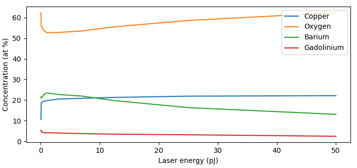
At a glance, the composition is relatively insensitive to the laser energy above ~25pJ. Below this laser energy the oxygen and copper decrease at %, where gadolinium and barium increase. This changes again below ~3pJ causing oxygen to quickly increase and barium to quickly decrease. This captures the essence of this computation, remembering that the whole mass spectrum should be ranged for this computation, which was not done for simplicity.