Multiple detection events
Detection cycles are partially characterized by a “multiplicity”. There is a non-zero probability that multiple ions can be detected during a single cycle (cycle meaning the time between two successive pulses). For some materials, even the majority of ions can be detected in such a fashion. The phenomenon is important and can have far reaching implications.
High proportions of multiple detection events can have invisible effects on mass spectrum analysis, due to generational changes in hit-finding, ion loss due to detector pile up, or displacement of mass/charge and position through molecular dissociation, among other things. This phenomena is most important in non-metals which are more prone to the effect than metals. APAV supports a few ways of studying these multiple detection events.
Correlation histograms
A correlation histogram is 2-dimensional histogram computed by aggregating ion pairs of a particular (or all) multiplicity and computing the histogram of ion 1 vs ion 2 of all ion pairs. In experiments with large fraction of multiple events these histograms can reveal the presence of multiple event related phenomena that can introduce aberrations into the mass analysis (such as molecular dissociation, generation of neutrals, or post-field ionization).
Important
If no dissociation tracks are present in a correlation histogram, this does not necessarily mean that the phenomenon did not occur. Instruments employing energy-compensating reflectrons can correct for some of these deviations but hide others. Neutrals generated prior to reflctron lensing will not be visible in any way.
A basic correlation histogram can be computed by:
>>> from apav import Roi
>>> from apav.analysis import CorrelationHistogram
>>> roi = Roi.from_epos("GBCO.epos")
>>> corr = CorrelationHistogram(roi)
The raw histogram can be retrieved via
>>> corr.histogram
array([[ 7., 12.,  8., ...,  0.,  0.,  0.],
   [ 0.,  7.,  2., ...,  0.,  0.,  0.],
   [ 0.,  0.,  3., ...,  0.,  0.,  0.],
   ...,
   [ 0.,  0.,  0., ...,  0.,  0.,  0.],
   [ 0.,  0.,  0., ...,  0.,  0.,  0.],
   [ 0.,  0.,  0., ...,  0.,  0.,  0.]])
The MultipleEventExtractor instance responsible for computing the ion pairs can be accessed with:
>>> corr.event_extractor
<apav.core.multipleevent.MultipleEventExtractor at 0x20bd5e62208>
Save the raw histogram using:
>>> corr.export("/path/to/output.csv")
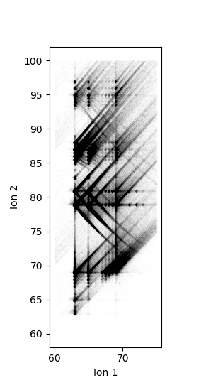
More details and arguments can be seen in the CorrelationHistogram API reference. A more detailed example. This computes and plots a correlation histogram for the GBCO experiment. It is computed for ion 1 between 60-75 Da and ion 2 from 60-100 Da:
>>> # APAV imports
>>> from apav import Roi
>>> from apav.analysis import CorrelationHistogram

>>> # matplotlib imports
>>> import matplotlib.pyplot as plt
>>> from matplotlib.colors import LogNorm
>>> from itertools import chain

>>> # Load the Roi and compute the correlation histogram
>>> roi = Roi.from_epos("GBCO.epos")
>>> corr = CorrelationHistogram(roi, extents=((60, 75), (60, 100)))

>>> # Adjust the raw histogram so we can display it with matplotlib properly
>>> hist = n.flipud(corr.histogram.T)

>>> # Generate the figure
>>> fig, ax = plt.subplots()
>>> extents = tuple(chain.from_iterable(corr.extents))
>>> im = ax.imshow(hist, aspect="equal", norm=LogNorm(), extent=extents)
>>> ax.set_xlabel("Ion 1")
>>> ax.set_ylabel("Ion 2")
>>> fig.colorbar(im, ax=ax)
>>> plt.show()
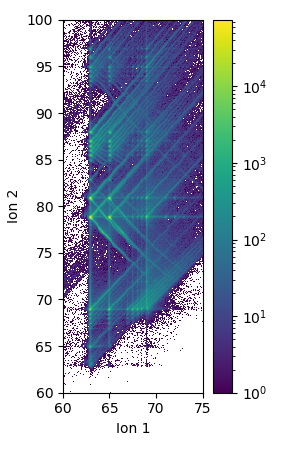
The raw histogram from CorrelationHistogram.histogram follows the matrix notation order for axes. I.e. the first axis (ion 1) is on the vertical and second axis (ion 2) on the horizontal. However, this is the opposite of what one may expect to see in a typical graph, this is why the raw histogram was transposed. Most plotting libraries also put the origin in the upper left corner for 2D image plots, where most graphs have the origin at the bottom left. This is why the raw histogram was flipped vertically. Both of the transforms are performed in the hist = n.flipud(corr.histogram.T) line - the order matters here.
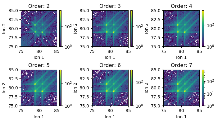
The multiplicity can be easily varied. Below we compute 6 symmetric correlation histograms of multiplicity 2-7 showing the dissipation of a dissociation track with high order multiplicity:
>>> # APAV imports
>>> from apav import Roi
>>> from apav.analysis import CorrelationHistogram

>>> # matplotlib imports
>>> import matplotlib.pyplot as plt
>>> from matplotlib.colors import LogNorm
>>> from itertools import chain

>>> # Load the Roi and compute the correlation histogram
>>> roi = Roi.from_epos("GBCO.epos")

>>> # Compute the histograms on an area with a dissociation track
>>> extents = ((75, 85), (75, 85))
>>> fig, axes = plt.subplots(2, 3)
>>> for idx, mult in enumerate(range(2, 8)):
>>>     i = idx // 3
>>>     j = idx % 3
>>>     corr = CorrelationHistogram(roi, extents=extents, multiplicity=mult)
>>>     hist = n.flipud(corr.histogram.T)
>>>     im = axes[i, j].imshow(hist, norm=LogNorm(), extent=tuple(chain.from_iterable(extents)))
>>>     fig.colorbar(im, ax=axes[i, j])
>>>     axes[i, j].set_xlabel("Ion 1")
>>>     axes[i, j].set_ylabel("Ion 2")
>>>     axes[i, j].set_title("Order: {}".format(mult))
>>> plt.show()
Interactive plotting
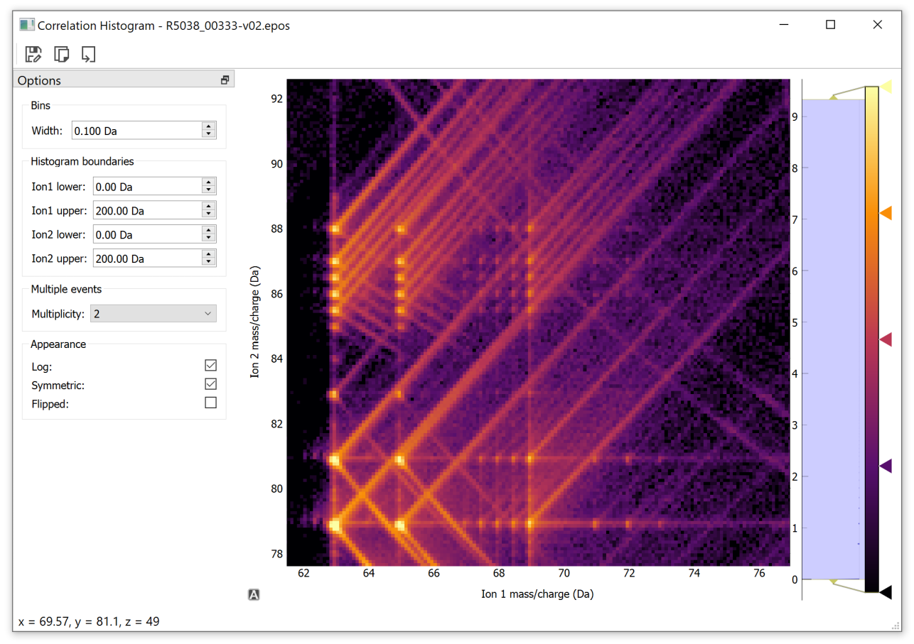
Alternatively, correlation histograms can be constructed interactively using a custom Qt widget with CorrelationHistogram.plot(). For example:
>>> from apav import Roi
>>> from apav.analysis import CorrelationHistogram
>>> roi = Roi.from_epos("GBCO.epos")
>>> corr = CorrelationHistogram(roi)
>>> plot = corr.plot()
>>> plot.show()
The resulting window is shown below (after some interaction). The interactive window includes controls for changing the bin width, histogram boundaries, multiplicity, log scale, histogram symmetry and histogram transposition. Right clicking the image brings up a context menu where the interaction style can be changed if the interaction is through a trackpad or mouse. The toolbar buttons allow the image to be saved to a file, copied to the system clip board, or the raw data to be saved to a csv. The raw data is saved as a text image (see CorrelationHistogram.export()) and the file name is automatically filled with a string indicating the x/y boundaries and bin width for future reference.
The colormap may be changed by right clicking on the colorbar itself. Individual points along the color bar can be adjust or color changed. The color map extents can be adjusted by dragging the rectangle next to the bar.
Note
Exporting the histogram as raw csv data saves the histogram in its natural format (with the origin in the upper left corner). It may need to be transformed (transposed then flipped) depending on intended usage.
Extracting multiple detection events
A class named MultipleEventExtractor is the entry point used for extracting ion pairs from the multiple events of an Roi. Most analyses using multiple events will use this class internally. This may also be used as an interface for producing custom analysis involving multiple event ion pairs.
Instantiate a MultipleEventExtractor as:
>>> from apav import Roi, MultipleEventExtractor
>>> roi = Roi.from_epos("/path/to/data.epos")
>>> mevents = MultipleEventExtractor(roi, 2)
Which creates a new MultipleEventExtractor instance containing information pertaining to the 2nd-order multiplicity ion pairs from the roi. The array of pairs themselves may be accessed through:
>>> mevents.pairs
array([[ 1.2204628 , 88.05748749],
       [34.98926163, 69.21746826],
       [63.23685455, 78.51170349],
       ...,
       [ 2.01867962, 63.52433395],
       [64.92139435, 78.54881287],
       [11.55757809, 20.1860199 ]])
This interface could be used to build correlation histograms in alternative ways. Sometimes ion pair correlations are represented as normal scatter plots, which might be useful if their ion counts are low:
>>> from apav.multipleevent import MultipleEventExtractor, Roi
>>> import matplotlib.pyplot as plt

>>> # Load the data
>>> roi = Roi.from_epos("GBCO.epos")

>>> # Extract multiple events of 2nd order where ion 1 is
>>> # between 60-75 Da and ion2 between 60-100 Da
>>> mevents = MultipleEventExtractor(roi, 2, extents=((60, 75), (60, 100)))

>>> # Plot a scatter plot of the ion pairs
>>> fig, ax = plt.subplots()
>>> ax.plot(mevents.pairs[::2, 0], mevents.pairs[::2, 1],
        "black", marker=".", markersize=0.01, linestyle="none")
>>> ax.set_xlabel("Ion 1")
>>> ax.set_ylabel("Ion 2")
>>> ax.set_aspect("equal")
>>> plt.show()
Example: Kinetic energy release
The MultipleEventExtractor also provides the indices of each ion in each ion pair, which acts as a mapping from each ion pair to the original Roi data (or any other relevant data for that matter). This allows any data in Roi.xyz, Roi.mass, or any other structured data in Roi.misc to be mapped to each ion pair. This way, more custom analysis can be done using multiple event pairs that may be less common.
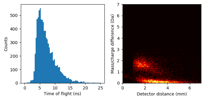
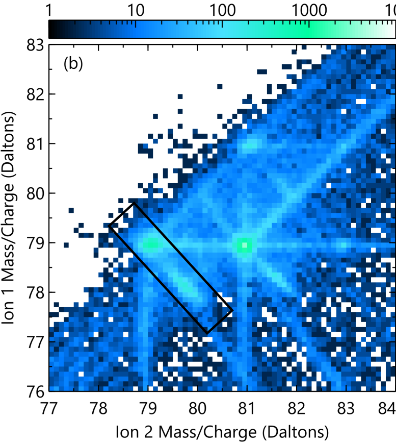
For example we will examine the molecular dissociation reaction of Cu2O2 2+ -> CuO+ + CuO +. Upon dissociation the products of this reaction “push away” from each other through a coulombic repulsion. This results in a kinetic energy loss that perturbs the TOF of both ions and the reconstruction positions. We can construct a mass/charge ratio vs detector distance plot to examine the effects on mass/charge displacement and reconstructed position (a factor of molecular orientation). Also we make a histogram of the TOF pair difference, allowing us to determine the dead time of the detector (~3.5 ns in LEAP 5000 XS instruments).
The dissociation track for this process is presented below, specifically the short lobes and not the long tracks. We will show how to make a mass/charge difference vs detector displacement histogram of all ion pairs just in the rotated black rectangle (shown below):
First load the data and extract the ion pairs:
>>> from apav import Roi, MultipleEventExtractor
>>> roi = Roi.from_epos("GBCO.epos")

>>> # Extract all multiple events
>>> mevents = MultipleEventExtractor(roi, "multiples")  # Use all multiple events
Next filter out all ion pairs that are not within the contained area. We are taking the end points of the rectangle as (ion1, ion2) = (79.5, 78.5) Da and (77.5, 80.5) Da, and the width as 0.5 Da. To do this we must transform the coordinate system to a more agreeable coordinate system to more easily with. We will translate one end of the rectangle to the origin (0, 0) and the rotate so the rectangle is horizontal:
>>> import numpy.linalg as la
>>> import numpy as n

>>> a = n.array([79.5, 78.5, 1])  # Rectangle end point 1 in homogeneous coordinates
>>> b = n.array([77.5, 80.5, 1])  # Rectangle end point 2 in homogeneous coordinates
>>> w = 0.5  # Rectangle width
>>> r = la.norm(b-a)  # Rectangle length

>>> dx = b[0] - a[0]  # X component of rectangle
>>> dy = b[1] - a[1]  # y component of rectangle

>>> # Calculate the rotation angle needed to make the rectangle horizontal
>>> theta = n.arctan(dy/dx)
>>> if theta < 0:
>>>     theta += n.pi

>>> # Construct the rotation transformation
>>> rotT = n.array([[n.cos(-theta), -n.sin(-theta), 0],
>>>                 [n.sin(-theta), n.cos(-theta),  0],
>>>                 [0,             0,              1]])

>>> # Construct the translation transformation
>>> transT = n.array([[1, 0, -a[0]],
>>>                   [0, 1, -a[1]],
>>>                   [0, 0,    1]])

>>> # Combine the transformations (order matters)
>>> T = rotT @ transT
Now that we have the transformation T ready, calculate the indices for ion pairs located in the rectangle roi:
>>> idx = mevents.pair_indices
>>> mass = data.mass[idx]

>>> # We must work in homogenous coordinates due to the translation transformation, so append a column of ones
>>> mass_hom = n.hstack([mass, n.ones([mass.shape[0], 1])])

>>> # Apply the transformation and drop off the extra column of ones
>>> transformed = (T @ mass_hom.T).T[:, 0:2]

>>> # Now filter out pairs that are not contained within the rectangle
>>> idx2 = n.argwhere((transformed[:, 0] >= 0) &
>>>               (transformed[:, 0] <= r) &
>>>               (transformed[:, 1] >= -w/2) &
>>>               (transformed[:, 1] <= w/2))[:, 0]

>>> # This is the array of all pairs contained within the rectangle
>>> idx_filt = idx[idx2]
Now use the filtered ion pair indices to retrieve the pair data from within the rectangle and make the plots:
>>> # Filtered mass/charge ratios, TOF, and detector coordinate info
>>> mass_filt = roi.mass[idx_filt]
>>> tof_filt = roi.mass[idx_filt]
>>> detx = roi.misc["det_x"][idx_filt]
>>> dety = roi.misc["det_y"][idx_filt]

>>> diff_detx = detx[:, 1] - detx[:, 0]
>>> diff_dety = dety[:, 1] - dety[:, 0]
>>> diff_det = n.sqrt(diff_detx**2 + diff_dety**2)
>>> diff_mass = n.diff(mass).ravel()
>>> diff_tof = n.diff(tof)

>>> # Plot the data
>>> fig, ax = plt.subplots(1, 2)
>>> ax[0].hist(diff_tof, bins=75, range=(0, 25))
>>> ax[0].set_xlabel("Time of flight (ns)")
>>> ax[0].set_ylabel("Counts")

>>> hist = ax[1].hist2d(diff_det, diff_mass, bins=(100, 100), range=((0, 7), (0, 7)), cmap="hot")
>>> ax[1].set_xlabel("Detector distance (mm)")
>>> ax[1].set_ylabel("Mass/charge difference (Da)")
>>> ax[1].set_aspect("equal")
>>> plt.show()
Finally this produces the two graphs showing both the detector dead time ~3.5 ns (first figure) and the mass/charge ratio difference vs detector distance showing the effect of molecular dissociation orientation on TOF and position.
See this reference for explanation of the right figure:
I. Blum, L. Rigutti, F. Vurpillot, A. Vella, A. Gaillard, and B. Deconihout, “Dissociation Dynamics of Molecular Ions in High dc Electric Field,” J. Phys. Chem. A, vol. 120, no. 20, pp. 3654–3662, 2016.