Positional data
The Roi
The Roi class is the entry point for loading/manipulating/storing positional data from atom probe experiments. This stores x/y/z positional data, mass/charge ratios, TOF, detector coordinates, etc. Synthetic data may also be created using Roi. An Roi can be created from a file or by hand.
From file
To create an Roi from a pos file:
>>> import apav as ap
>>> data = ap.Roi.from_pos("data.pos")
By hand
An Roi can also be created by hand, perhaps for simulation purposes. As an example, lets create a simulated Cu-Al interface that is slightly diffused. Starting with the imports and setup:
>>> import numpy as n
>>> import apav as ap
>>> rand = n.random.default_rng()
Create the Cu and Al positions:
>>> cu_pos = rand.uniform((-20, -20, -20), (20, 20, 0), (1000, 3))
>>> al_pos = rand.uniform((-20, -20, 0), (20, 20, 20), (1000, 3))
Diffuse the interface using a normal distribution with standard deviation of 3nm only in the z-direction:
>>> cu_pos[:, 2] += rand.normal(0, 3, 1000)
>>> al_pos[:, 2] += rand.normal(0, 3, 1000)
>>> all_pos = n.vstack([cu_pos, al_pos])
Now the fake mass/charge ratios:
>>> mass = n.ones(2000)
>>> mass[:1000] = 63.5
>>> mass[1000:] = 27
Then creating the Roi is simply:
>>> roi = ap.Roi(all_pos, mass)
Basic properties
Note
Experimental datasets used in various code examples can be downloaded here: https://doi.org/10.5281/zenodo.7730641
Many properties of the Roi can be accessed using property getters. We will use the data from a LEAP experiment of a GdBa2Cu3O7 superconductor in both POS and ePOS format:
>>> from apav import Roi
>>> pos_roi = Roi.from_pos("GBCO.pos")
>>> epos_roi = Roi.from_pos("GBCO.epos")
The total number of ions/counts can be retrieved with:
>>> pos_roi.counts
73119146
The arrays of mass/charge ratios and atomic positions can be accessed by:
>>> " Mass/charge ratio array
>>> pos_roi.mass
array([ 33.390823,  32.75491 ,  64.936806, ..., 220.17    , 152.62997 ,
   116.74453 ], dtype=float32)

>>> " x/y/z ion position array
>>> pos_roi.xyz
array([[  9.837536,  -7.579013,   3.344986],
   [ 11.597513, -10.081262,   5.355319],
   [ 11.67127 ,  -9.669364,   5.190416],
   ...,
   [-24.225286,  26.560808, 604.4885  ],
   [-19.90658 ,  35.445568, 606.35614 ],
   [ 21.92588 ,  20.546566, 602.50946 ]], dtype=float32)
Optional structured data loaded from external files can be accessed from the Roi.misc dictionary:
>>> epos_roi.misc
{'tof': array([ 653.6501,  658.9791,  926.4651, ..., 1232.3171, 1030.2881,
         885.5371], dtype=float32),
 'dc_voltage': array([3804.03, 3804.03, 3804.03, ..., 6920.98, 6920.98, 6924.98],
       dtype=float32),
 'pulse_voltage': array([0., 0., 0., ..., 0., 0., 0.], dtype=float32),
 'det_x': array([ 18.250248,  22.35933 ,  22.507404, ..., -14.548371, -12.475321,
          8.033071], dtype=float32),
 'det_y': array([-16.553726, -22.180542, -21.272991, ...,  12.633107,  17.13456 ,
          9.583736], dtype=float32),
 'psl': array([949201,      0,      0, ...,   8475,   2784,   9007]),
 'ipp': array([5, 0, 0, ..., 1, 1, 1], dtype=uint8)}
See the below Units section for more detail on the miscellaneous data. Some properties of the atom position distribution can be accessed, such the center, boundaries, dimensions, etc:
>>> # The length/width/height of all positions
>>> pos_roi.dimensions
array([[131.85028076],
   [133.37796021],
   [622.87325295]])

>>> # The boundaries of all positions
>>> pos_roi.xyz_extents
((-66.83065032958984, 65.0196304321289),
 (-66.87464141845703, 66.5033187866211),
 (0.03708640858530998, 622.9103393554688))

>>> # The center of all positions (average of x, y, and z)
>>> pos_roi.xyz_center
array([  0.5118104,  -0.7339013, 234.95718  ], dtype=float32)
The min/max of the mass distribution may also be queried, though due to noise the max value here can be quite high:
>>> pos_roi.mass_exents
(0.013478817, 2178.0952)
Units
Structured data of common properties in the Roi class are expected to be in certain units. If the data was loaded from external files such as POS, ePOS, ATO, or APT then the units are automatically converted. Otherwise the table below shows both the expected units as well as the accessor. Not all of these properties are always present (or used) in a given file formats. Nevertheless, they are read from POS/ePOS/ATO files so as to be accessible.
See here for technical details of these properties.
Property |
Unit |
Roi accessor |
|---|---|---|
Mass/charge |
Daltons (Da) |
|
X/Y/Z |
Nanometers (nm) |
|
Detector coordinates |
Millimeters (mm) |
|
Time of flight |
Nanoseconds (ns) |
|
Voltages |
Volts (V) |
|
Ions/pulse |
|
Synthetic data
The default Roi constructor can be used to deliberately create an atom probe dataset using data from whatever means. The restrictions are:
At least 1 atomic position must be supplied including its x, y, z, and its mass/charge ratio
xyz coordinates are provided as a 2-dimensional array
Mass/charge ratios are provided as a 1-dimensional array
For example:
>>> from apav import Roi
>>> import numpy as np
>>>
>>> xyz = n.array([[0, 0, 0]])
>>> mass = n.array([6])
>>> fake_roi = Roi(xyz, mass)
Creates a new Roi object containing 1 carbon atom located (0, 0, 0) with a mass/charge ratio m/n =12 Da. Or less trivially:
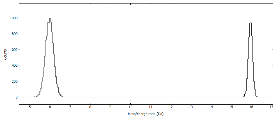
>>> import numpy as np
>>> from apav import Roi
>>> mass_C = np.random.normal(6, 0.2, 10000)
>>> mass_O = np.random.normal(16, 0.1, 5000)
>>> mass = np.concatenate([mass_C, mass_O])
>>> xyz = n.random.random([15000, 3])*10
>>> roi = Roi(xyz, mass)
Which produces 15,000 atom positions, 10,000 carbon atoms and 5,000 oxygen atoms. The XYZ positions are randomly distributed in a 10x10x10 nm box. The mass/charge ratios for C are distributed along a normal distribution centered at 6 Da with a 0.2 standard deviation, the oxygen mass ratios are also distributed in a normal distribution centered on 16 Da with a 0.1 standard deviation. roi.plot_mass_histogram() gives:
Multiple events
Handling multiple events are somewhat more nuanced as the Roi may or may not contain the data necessary to process multiple events - it depends on how the Roi was constructed. APAV follows the same designation as the ePOS file format for storing multiple event data - “ions per pulse”. If the Roi contains this array in its miscellaneous dict as Roi.misc["ipp"] then the Roi can be used for multiple event related processing.
Note
The “ions per pulse” array is a 1-dimensional array with a single entry for each atom. Non-zero entries indicate the number ions that were detected between the pulse of that atom and the next pulse. So 1 “ions per pulse” indicate a single event, 3 “ions per pulse” indicate 3 ions before the next pulse. Entries >= 2 are followed by null entries, indicating each subsequent ion as part of that multiple event. Take the ion sequence below:
Ion # |
Ions/pulse |
Mass/charge |
|---|---|---|
1 |
1 |
12 |
2 |
1 |
45 |
3 |
2 |
23 |
4 |
0 |
24 |
5 |
5 |
124 |
6 |
0 |
125 |
7 |
0 |
11 |
8 |
0 |
130 |
9 |
0 |
5 |
Ion #1 and #2 are single events, only 1 ion detected between pulses. Ion #3 starts a multiple event with 2 ions detected between pulses, where ion #3 was the first ion and ion #4 the second, this produces the ion pair of masses (23, 24) Da. Ion #5 starts a multiple event with 5 ions detected between pulses. This is followed by 4 null entries forming the 5-ion sequence (124, 125, 11, 130, 5) Da.
If multiple event information is available (which can be checked if unsure by Roi.has_multiplicity_info()) then some additional information regarding the multiple event character of the Roi can be accessed. The sorted multiplicity orders can be accessed:
>>> epos_roi.multiplicities
array([ 1,  2,  3,  4,  5,  6,  7,  8,  9, 10, 11, 12, 13, 14, 15],
  dtype=int64)
Which indicates that the GBCO.epos experiment produced up to at least a single 15th order multiple event. The proportion of counts in each multiplicity order can be determined:
>>> # Total multiplicity counts per order
>>> epos_roi.multiplicity_counts
(array([ 1,  2,  3,  4,  5,  6,  7,  8,  9, 10, 11, 12, 13, 14, 15],
       dtype=int64),
 array([3.7978187e+07, 1.2674826e+07, 7.7557890e+06, 4.7011600e+06,
        3.1888200e+06, 2.2440540e+06, 1.7141810e+06, 1.5814560e+06,
        1.0828440e+06, 1.8250000e+05, 1.1748000e+04, 2.0280000e+03,
        8.8400000e+02, 5.0400000e+02, 1.6500000e+02]))

>>> # Multiplicity counts in percentage
>>> epos_roi.multiplicity_percentage
(array([ 1,  2,  3,  4,  5,  6,  7,  8,  9, 10, 11, 12, 13, 14, 15],
   dtype=int64),
 array([5.19401403e+01, 1.73344831e+01, 1.06070563e+01, 6.42945146e+00,
        4.36112862e+00, 3.06903749e+00, 2.34436682e+00, 2.16284802e+00,
        1.48093086e+00, 2.49592631e-01, 1.60669273e-02, 2.77355537e-03,
        1.20898567e-03, 6.89285950e-04, 2.25659091e-04]))

>>> # Multiplicity counts in proportion
>>> epos_roi.multiplicity_fraction
Here we can see that only 165 out of the 73,119,146 counts are of 15th order, or that 51.9% of counts are single events. If we attempt to access this information from a Roi that does not have multiple event information we get an error:
>>> pos_roi.multiplicities
---------------------------------------------------------------------------
NoMultiEventError                           Traceback (most recent call last)
<ipython-input-19-1ff141533db1> in <module>
----> 1 roi2.multiplicities

~\PycharmProjects\apav\apav\core\roi.py in multiplicities(self)
    101     def multiplicities(self) -> ndarray:
    102         if not self.has_multiplicity_info():
--> 103             raise NoMultiEventError()
    104         elif self.has_multiplicity_info() and self._multiplicities is None:
    105             self._multiplicities = unique_int8(self.misc["ipp"])

NoMultiEventError: Roi has no multiple-hit information
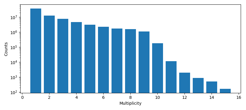
For example, we can use this information to plot the distribution of multiplicity vs counts:
>>> import matplotlib.pyplot as plt
>>> mults, counts = epos_roi.multiplicity_counts()
>>> plot.bar(mults, counts, log=True)
>>> plt.xlabel("Multiplicity")
>>> plt.ylabel("Counts")
>>> plt.show()
Roi subsets
Those familiar with the the commercial software IVAS (from Cameca) may recall the concept of a ROI referring to a subset of data “cropped” by geometric primitives such as a sphere, cylinder, or rectangular prism. APAV offers similar functionality by use of RoiSubsetType subclass. APAV offers the same basic primitives for this function: RoiSphere, RoiCylinder, and RoiRectPrism.
Note
Currently neither the RoiCylinder or RoiRectPrism can be rotated. The RoiCylinder can, however, be aligned in either major axis x, y, or z.
Lets imagine there is a spherical precipitate in GBCO.epos located at the center (13.4, 25.6, 486.3) nm with an approximate diameter of 21nm. We could retrieve the mass spectrum composed of all multiple events of this precipitate by simply using RoiSphere:
>>> from apav import Roi, RoiSphere
>>> roi = Roi.from_epos("GBCO.epos")
>>> precip_roi = RoSphere(roi, (13.4, 25.6, 486.3), 10)
>>> mass_histogram = precip_roi.mass_histogram(multiplicity="multiples")
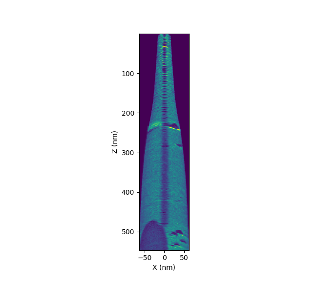
A density map of a 3nm slice of the XZ plane axis using RoiRectPrism:
>>> # Create the Roi
>>> import apav as ap
>>> roi = ap.Roi.from_pos("GBCO.pos")

>>> # Create the Roi slice
>>> dx, dy, dz = roi.dimensions
>>> slice_roi = RoiRectPrism(roi, roi.xyz_center, (dx, 3, dz))

>>> # Create the density map and plot it
>>> fig, ax = plt.subplots()
>>> ax.hist2d(slice_roi.xyz[:, 0], slice_roi.xyz[:, 2], bins=(50, 300))
>>> fig.gca().invert_yaxis()
>>> ax.set_aspect("equal")
>>> ax.set_xlabel("X (nm)")
>>> ax.set_ylabel("Z (nm)")
>>> plt.show()
This creates the figure:
A final example for RoiCylinder. We notice the low density region in the previous figure which often indicates a region of atomic plane resolution. We can plot a 1D histogram through this pole using a cylinder centered at (0, 0, 350) nm with a height and radius of 50nm and 5 nm, respectively:
>>> # Create the Roi
>>> import apav as ap
>>> roi = ap.Roi.from_pos("GBCO.pos")

>>> # Create the cylinder Roi
>>> dx, dy, dz = roi.dimensions
>>> cyl_roi = RoiCylinder(roi, (0, 0, 350), 5, 50)

>>> # Create the histogram and plot it
>>> plt.hist(roi_cyl.xyz[:, 2], bins=1000)
>>> plt.xlabel("Z (nm)")
>>> plt.ylabel("Counts")
>>> plt.show()
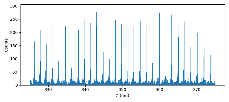
This particular Z-histogram is not particularly useful, conventional atomic plane analysis typically uses spatial distribution maps - though this captures the essence of RoiCylinder usage.
Note
Each RoiSubsetType does not copy data from the parent Roi. This would otherwise greatly increase
the memory cost of using these classes. Each RoiSubsetType instead keeps an array for indexing into
the parent Roi.
Mass/TOF spectra
TOF spectra (if the data is available) is accessed through Roi.tof_histogram() and mass spectra through Roi.mass_histogram() see the API reference for argument details. Both spectra have arguments for changing the bin width, spectrum boundaries, normalization, and multiplicity.
Important
The TOF data saved in epos files through IVAS is the uncorrected TOF, not the voltage/bowl corrected TOF. Those interested in TOF analysis should pursue *.apt files as they can embed different TOF corrections.
For an example, we will compute 2 figures of GBCO: the mass histograms for the single/multiple events 1-5 and the mass histograms for all counts, single events, and all multiple events:
>>> from apav import Roi
>>> import matplotlib.pyplot as plt
>>> roi = Roi.from_epos("GBCO.epos")

>>> fig, axes = plt.subplots(1, 2)

>>> # Mass spectra lower and upper bounds
>>> low = 60  # Da
>>> high = 90  # Da

>>> # Compute the mass histograms for multiplicity order 1 through 5 and plot
>>> for i in range(1, 6):
>>>     centers, counts = roi.mass_histogram(lower=low, upper=high, multiplicity=i)
>>>     axes[0].plot(centers, counts, label=str(i), linewidth=1)

>>> # Figure settings
>>> axes[0].set_yscale("log")
>>> axes[0].legend()
>>> axes[0].set_xlabel("Mass/Charge Ratio (Da)")
>>> axes[0].set_ylabel("Counts")

>>> # Compute the mass histograms for all counts, single events, and all multiples
>>> all_hist = roi.mass_histogram(lower=low, upper=high, multiplicity="all")
>>> singles_hist = roi.mass_histogram(lower=low, upper=high, multiplicity=1)
>>> multiples_hist = roi.mass_histogram(lower=low, upper=high, multiplicity="multiples")

>>> # Plot the histograms
>>> axes[1].plot(all_hist[0], all_hist[1], label="All", linewidth=1)
>>> axes[1].plot(singles_hist[0], singles_hist[1], label="Singles", linewidth=1)
>>> axes[1].plot(multiples_hist[0], multiples_hist[1], label="Multiples", linewidth=1)

>>> # Figure settings
>>> axes[1].set_yscale("log")
>>> axes[1].legend()
>>> axes[1].set_xlabel("Mass/Charge Ratio (Da)")
>>> axes[1].set_ylabel("Counts")

>>> # Show the figure
>>> plt.show()
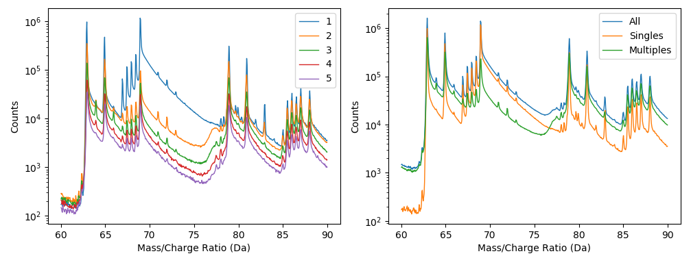
Such plots can give some indication of mass spectrum aberrations arrising from multiple event related phenomena. The region from 75 - 77 Da has a drastic difference between the single events and multiple events. This difference in leading edges of this isotope may be an indication of molecular dissociation. The dissipation of the leading edge “hump” after the 2nd order multiplicity may represent the number of products associated with the dissociation.
Interactive plotting
Alternatively, the mass spectra of an Roi may be explored interactively using Roi.plot_mass_spectrum() allowing quick exploration of an experimental mass spectrum. The example below shows this window displaying the mass spectrum of GBCO using only 6th order multiple events. The buttons in the top left of the toolbar allow for interactively saving an image, copying the image to the clipboard, and exporting raw data, respectively:
>>> %gui qt
>>> import apav as ap
>>> roi = ap.Roi.from_pos("GBCO.pos")
>>> plot = roi.plot_mass_spectrum()
>>> plot.show()
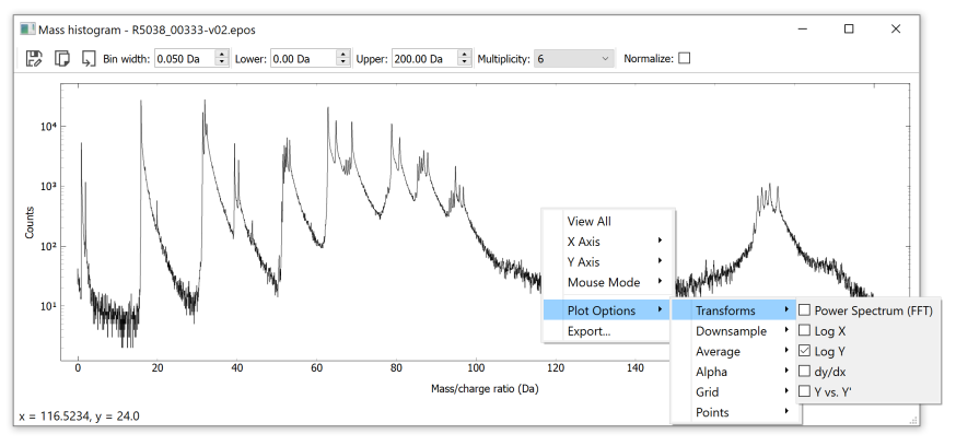
The context menu (right click) is a function of pyqtgraph, options here are sometimes buggy (your mileage may vary).