Spatial analysis
Spatial analysis in APT is a very interactive process, typically requiring multiple iterations of manual parameter refinement and visual assessment. Because of this, APAV has limited 3D spatial analysis capability (APAV does not currently have a global user interface for easily tuning 3D parameters). Still, APAV does provide classes for calculation of compositional grids which is non-trivial, but enough to provide a backbone for custom analysis.
Compositional grids
Many spatial analysis in APT begins with the computation of “compositional grids”, a process where the spatial domain of the dataset is divided into a 3D grid and each (ranged) ion is placed into a voxel. Each range composition has their own grid, which allows for calculation of the composition at each voxel. Such a grid-based compositional representation can enable other common analyses such as volume rendering, iso-concentration contours, proximity histograms, etc.
Calculation of the grids is non-trivial due to each ion being delocalized from the center of any bin. Standard process (in IVAS or AP Suite) is to perform this calculation in stages, cumulatively referred to as delocalization.
Delocalization
The first pass of delocalization places each ion into the initially empty bins. Computationally, this process is slow due to the unstructured/random positions of ions (i.e. no FFT or other accelerations are available). Further, each ion is a real, physical object that can potentially intersect more than its closest bin. Due to this delocalization and physical size, we distribute every ion among its closest bin and each neighboring bin. The internal implementation of this function is a multithreaded c extension to get as much performance as possible.
The second pass of delocalization smooths each image (3D grid) to reduce noise and outliers during ensuing use of the grids.
In APAV we follow as close as we can to the delocalization behavior in IVAS/AP Suite for compatibility purposes. Delocalization is defined as a single parameter for each cardinal direction, which expresses the degree of “delocalization” or smoothing in that direction. Both delocalization passes use normal distributions, so each delocalization parameter relates to the standard deviation of the cumulative delocalization of each pass (in the given direction). Specifically, the delocalization in the x-axis, \(d_x\), expresses the total \(3\sigma\) spread such that the standard deviations in each pass are added in quadrature, i.e., \(d_x=3\sigma_x=\sqrt{(3\sigma_{x1})^2+(3\sigma_{x2})^2}\) (\(\sigma_{x1}\) is the first pass standard deviation and \(\sigma_{x2}\) the second pass). The \(3\sigma\) standard deviation of the first pass gaussian transfer function is set to half the bin width, i.e., \(3\sigma_1=b/2\). The standard deviation of the second pass gaussian kernel is determined by the remaining length in the delocalization.
For example, if \(d_x=4\) nm and the bin width is 0.5 nm, then \(3\sigma_{x1}=0.5/2\) nm or a first-pass standard deviation of \(\sigma_{x1}=0.0833\) nm. The standard deviation in the second-pass gaussian kernel is the remaining distance as determined by \(4=\sqrt{(3\times0.0833)^2+(3\sigma_{x2})^2}\) which becomes \(\sigma_{x2}=2.31\) nm. As mentioned, this process follows what is known about IVAS/AP Suite.
Note
The default delocalization is \(3\times3\times1.5\) nm, but can be changed.
The delocalization value can vary for each cardinal direction, but conventionally the delocalization is the same in the x/y directions and smaller in the z. The z-axis delocalization tends to be smaller due to the better spatial resolution in this direction (remember that the z coordinate is determined by the time-of-flight and the x/y coordinates by the detector position).
Using ranged grids
Calculation of compositional grids is provided by the RangedGrid class. Below is a full example of loading data, creating the ranged grid, and plotting concentration maps:
>>> # Imports
>>> import apav as ap
>>> import apav.analysis as anl
>>> import matplotlib.pyplot as plt
>>> # Load data
>>> roi = ap.load_epos("R5038_00556-v04.epos")
>>> rng = ap.load_rrng("rng_5pj.rrng")
>>> # Create the ranged grids using 0.5 nm bin width and default delocalization
>>> grids = anl.RangedGrid(roi, rng, bin_width=0.5)
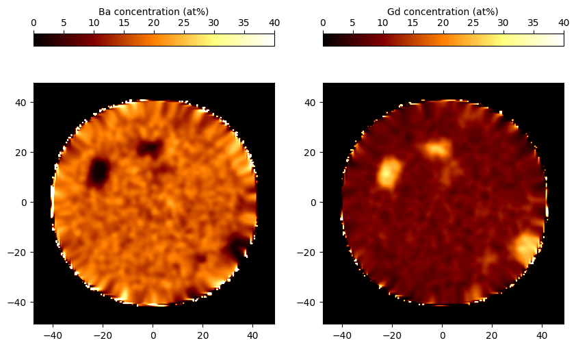
>>> # Plot a slice
>>> Ba = grids.elemental_frac("Ba") * 100
>>> Gd = grids.elemental_frac("Gd") * 100
>>> Ba_slice = Ba[:, :, 276]
>>> Gd_slice = Gd[:, :, 276]
>>> extents = (*grids.extents[0], *grids.extents[1])
>>> fig, ax = plt.subplots(1, 2)
>>> img1 = ax[0].imshow(Ba_slice, vmin=0, vmax=40, extent=extents, cmap="afmhot")
>>> img2 = ax[1].imshow(Gd_slice, vmin=0, vmax=40, extent=extents, cmap="afmhot")
>>> color = plt.colorbar(img1, location="top", ax=ax[0])
>>> color.set_label("Ba concentration (at%)")
>>> color2 = plt.colorbar(img2, location="top", ax=ax[1])
>>> color2.set_label("Gd concentration (at%)")
>>> plt.show()
The first pass delocalization can be disabled in the constructor using the first_pass flag, i.e. RangedGrid(roi, rng, first_pass=False). This is equivalent to assigning each ion entirely to the nearest bin and applying the whole delocalization distance to the gaussian smoothing.
Multivariate histograms
We can easily get a sense for what phases might be present by analyzing the statistical correlation in the grid-based voxel concentrations. In the example below we continue from the previous example and plot a bivariate histogram correlating the Ba-Gd concentrations:
>>> counts = grids.elemental_counts_grid
>>> mask = counts.ravel() > 1
>>> gd_list = Gd.ravel()[mask]
>>> ba_list = Ba.ravel()[mask]

>>> hist = plt.hist2d(gd_list, ba_list, bins=100, vmax=2500)
>>> plt.xlabel("Gd concentration (at%)")
>>> plt.ylabel("Ba concentration (at%)")
>>> plt.show()
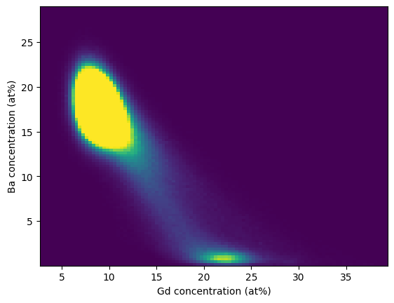
In this histogram we can trivially that some secondary phase is present that is Ba-deficient.