Getting started
The majority of APAV is split into 2 imports. The core import loads the main classes that represent data in APAV:
>>> import apav
Or more succinctly:
>>> import apav as ap
This brings in core containers such as Roi, Range, RangeCollection, and others. The second import loads most of the analysis processes, such as mass spectrum quantification routines, correlation histograms, density maps, etc:
>>> import apav.analysis
or shortened:
>>> import apav.analysis as anl
Importing data
Positional data
Positional data is stored and accessed in the Roi class. See the Roi page for detailed information. Loading positional data into Roi objects is done through its alternate constructors (i.e. @classmethod ) of the Roi object. For example, loading a POS file into a new Roi instance is simply:
>>> import apav as ap
>>> pos_roi = ap.Roi.from_pos(r"/path/to/data.pos")
Similarly for other file types:
>>> import apav as ap
>>> epos_roi = ap.Roi.from_epos(r"/path/to/data.epos")
>>> ato_roi = ap.Roi.from_ato(r"/path/to/data.ato")
The Roi instance can then be used directly, or passed to other analysis routines. There are also convenience functions functions that essential alias the Roi constructors, ie:
>>> import apav as ap
>>> data = ap.load_apt("data.apt")
Ranging data
Mass ranging uses the dedicated container RangeCollection, which can read RNG or RRNG files in the same manner as the Roi class with positional data. That is, through @classmethod alternate constructors. For example, loading a RRNG file of a Si material:
>>> import apav as ap
>>> rng = ap.RangeCollection.from_rng(r"/path/to/ranges.rng")
>>> rrng = ap.RangeCollection.from_rrng(r"/path/to/ranges.rrng")
Or for convenience:
>>> rng = ap.load_rng(r"path/to/ranges.rng")
We can print a summary of the RRNG file to check what it contains:
>>> print(rrng)
Range data set
Number of ranges: 25
Mass range: 5.896 - 86.555
Number of unique elements: 5
Elements: Si, Cu, C, O, Cr

Composition      Min (Da)    Max (Da)    Volume  Color (RGB 0-1)
-------------  ----------  ----------  --------  -----------------
C                  5.896        6.193   0.00878  (0.4, 0.0, 0.2)
C                 11.866       12.198   0.00878  (0.4, 0.0, 0.2)
Si                13.8745      14.241   0.02003  (0.8, 0.8, 0.8)
Si                14.407       14.643   0.02003  (0.8, 0.8, 0.8)
Si                14.912       15.171   0.02003  (0.8, 0.8, 0.8)
O2                15.858       16.48    0.02883  (0.0, 0.8, 1.0)
O2                17.838       18.304   0.02883  (0.0, 0.8, 1.0)
Cr                24.895       25.445   0.01201  (1.0, 0.2, 0.8)
Cr                25.771       27.211   0.01201  (1.0, 0.2, 0.8)
Si                27.856       28.595   0.02003  (0.8, 0.8, 0.8)
Si                28.826       29.255   0.02003  (0.8, 0.8, 0.8)
Si                29.783       30.252   0.02003  (0.8, 0.8, 0.8)
CrO               32.892       33.275   0.04083  (1.0, 0.0, 0.0)
CrO               33.898       34.802   0.04083  (1.0, 0.0, 0.0)
CrO               34.917       35.231   0.04083  (1.0, 0.0, 0.0)
CrO2              41.869       43.181   0.06966  (0.0, 1.0, 0.0)
Cr                49.612       50.526   0.01201  (1.0, 0.2, 0.8)
Cr                51.699       54.243   0.01201  (1.0, 0.2, 0.8)
Cr2O              57.819       61.159   0.05284  (0.0, 0.0, 1.0)
Cu                62.567       63.496   0.01181  (1.0, 0.4, 0.0)
Cu                64.619       65.548   0.01181  (1.0, 0.4, 0.0)
CrO               65.76        66.264   0.04083  (1.0, 0.0, 0.0)
CrO               67.622       69.574   0.04083  (1.0, 0.0, 0.0)
CrO               69.781       70.156   0.04083  (1.0, 0.0, 0.0)
CrO2              83.595       86.555   0.06966  (0.0, 1.0, 0.0)
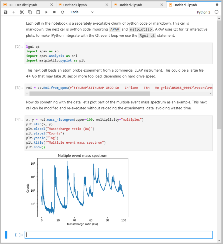
Jupyter Notebooks
APAV works in any IDE/code editor, however, Jupyter Lab is recommended due to the ability to segment code execution into “cells”. This is most advantageous when dealing with datasets with large number of counts where loading data could take longer than the analysis itself. The ability to separate data import from analysis can save much time when code needs to be adjusted and re-executed. See https://jupyter.org/ for more information about Jupyter Lab, it is installable straight from pip or conda.
See this example notebook:
Interactive plotting
Some classes in APAV can produce interactive plots. All of these integrated plots are interactive with the mouse. By default “right-click” and drag will scale/zoom the plot and “single-click” and drag will move the plot. This can be changed in the right-click menu to be more usable on trackpads. Many interactive plots in APAV also include edit fields where the analysis can be adjusted in real-time.
Important
When APAV is being used interactively, such as in a Jupyter Notebook or IPython session, the interpreter must
be told to integrate itself with the Qt event loop. Otherwise none of the interactive plots will work. This
simply fixed by inserting %gui qt at the top of the script.
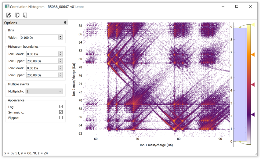
As an example, here is the interactive correlation histogram window. Note that the %gui qt statements is only required in interactive sessions such as notebooks or ipython sessions:
>>> %gui qt
>>> import apav as ap
>>> import apav.analysis as anl
>>> roi = ap.Roi.from_epos("data.epos")
>>> corr_hist = anl.CorrelationHistogram(roi)
>>> plot = corr_hist.plot()
>>> plot.show()
Note
Each interactive plot in APAV follows the same template, the plot function returns a Qt object which
must be assigned to an object or it will be garbage collected. Then the plot is shown using
some_plot.show().
For example, this is valid:
plot = some_analysis.some_plot_function()
plot.show()
This is not:
some_analysis.some_plot_function().show()